VRFB Stack Temperature Prediction

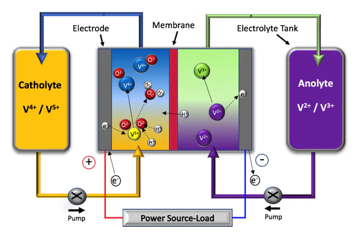
Redox Flow Batteries have risen in popularity in recent years as a large-scale energy storage solution. Efficiency of the battery storage system relies on minimizing power loss, which in turn is dependent on predicting VRFB stack temperature and keeping it within a safe limit so as to prevent thermal precipitation. We have predicted variation of stack temperature with time duration of a practical 1kW 6kWh VRFB system dataset under four different operating current levels (40, 45, 50, and 60A) keeping a constant electrolyte flow rate of 180 ml/sec for both charging and discharging conditions.

Here, we have used both Polynomial Regression and LSTM methods to accurately predict the stack temperature of the battery during charging and discharging profiles. The prediction accuracy of the algorithm was tested using regression metrics such as Root Mean Square Error (RMSE), Mean Absolute Error (MAE) and Correlation Coefficient (R2).

In the case of Polynomial Regression, we created models for degrees 0-9 and implemented it on the dataset. We used gradient descent to update the weights at each iteration. The MSE error was calculated every 5000 iterations and the model was run for a total of 50000 iterations.

For LSTM, We used the ‘train_test_split’ function within Scikit-learn to split the dataset 70:30 for training and testing respectively. We did not shuffle the data in this case as LSTM’s need sequential data for performing time series prediction. We reshaped the training and testing temperature data and performed Min-Max scaling using the ‘MinMaxScaler’ function within Scikit-learn so as to bring all temperature values within the range [0,1]. Min-Max scaling is performed when it is required to capture small variance in features and also for sparse data where the zero value needs to be preserved.

We then used the ‘TimeseriesGenerator’ module within Tensorflow to generate a time series with number of features as 1 and number of inputs as 5. Essentially this means that the model will use 5 values from the data to predict the 6th value in the data. We then created an LSTM model having 100 hidden layers which takes an input of shape (5,1) and uses a ReLU activation function at the output layer finally giving an output of size 1. The Adam optimizer with a learning rate of 0.001, β1 = 0.9, β2 = 0.999, ϵ = 10-8 was used with no weight decay. MSE error was used as the loss function.

The model was then trained on the training dataset for 50 epochs and the loss per epoch was plotted. We then used the model for prediction over the length of the entire dataset and the predicted values were stored in an array before being rescaled to the original size. The array was added later as an extra column within the dataset. The final MSE, RMSE and R2 errors were calculated and tabulated. We then plotted the algorithm performance and the parameter performance graphs.

For the obtained results and graphs, check out the paper!